
- Docs
- /
Data Tuning Advisor Algorithms
06 Jul 2020 39403 views 0 minutes to read Contributors ![]()
original source: https://www.microsoft.com/en-us/research/uploads/prod/2020/06/Anytime-Algorithm-of-Database-Tuning-Advisor-for-Microsoft-SQL-Server.pdf
Anytime Algorithm of Database Tuning Advisor for Microsoft SQL Server
Surajit Chaudhuri, Vivek Narasayya
Microsoft Research
June 2020
Abstract
This article provides an overview of the algorithm used by the Database Engine Tuning Advisor (DTA) in Microsoft SQL Server. While many aspects of these algorithms have been described in published papers, in this article we capture the algorithm end-to-end and include a few additional details. One goal of this article is to share with the database community the algorithm and make it easier for researchers intending to compare different approaches to physical design tuning. Note that several patents have been issued to Microsoft that protects its intellectual rights for commercial use of this algorithm.
Introduction
The Database Engine Tuning Advisor (DTA) is a physical design tool for Microsoft SQL Server. The first version of this tool (then called the Index Tuning Wizard [1]) was released in 1998 as part of Microsoft SQL Server 7.0 release. The tool evolved from a wizard to the application called DTA in Microsoft SQL Server 2005 [7]. DTA has been repeatedly updated in subsequent releases of the product, e.g., see [9] that describes some of the recent enhancements as part of SQL Server 2016 release. This algorithm is also the basis of Cloud version of the DTA used for tuning Azure SQL Database, that is in private preview [13, 14].
DTA takes as input one or more databases and a workload, consisting of a set of SQL statements (query, insert, update, delete), along with several constraints. These constraints include: a total storage bound, an allotted tuning time, a limit on the number of indexes per table, maximum number of columns in an index, a minimum required improvement for the workload etc. With each query in the workload, there is associated an optional user specified weight. By default, DTA uses the frequency of the query in the workload as its weight. The user may point DTA to an explicitly specified workload (e.g. a file of SQL statements) or implicitly by pointing to the Query Store [12], which contains the history of SQL statements that have executed against the database.
DTA produces as output a physical design configuration (i.e. set of physical design structures) such that the total query optimizer estimated cost of the workload is minimized. Typically, the total optimizer estimated cost is modeled as a sum (or a weighted sum) of costs of each query in the query but the core technique of DTA is not limited to only sum and weighted sum. The optimizer estimated cost of a query for a given configuration is obtained using a “What-If” API, which is an extended interface of the regular query optimizer of Microsoft SQL Server [2]. For each query in the workload, DTA returns the cost of the query in the current configuration as well as the recommended configuration, thereby allowing the user to better understand the impact of the proposed physical design.
DTA can recommend configurations consisting of several types of physical design structures:
- B+-Tree indexes including clustered and non-clustered indexes.
- Partial indexes (called Filtered Indexes). They are non-clustered, B+Tree indexes with filter
- Column store indexes. Unlike a B+Tree index, a columnstore index stores the data column-wise, thereby achieving greater compression and reduced I/O cost.
- Materialized Views (called Indexed Views). The class of materialized views considered is single-block Select-Project-Join with Group-By and Aggregation. Furthermore, clustered and non-clustered indexes can be created on a materialized view.
- Horizontal Partitioning. Heaps, clustered and non-clustered indexes can be horizontally partitioned using range partitioning functions. A non-clustered index can optionally be partition-aligned. This means the index is partitioned identically as the base table (i.e. heap/clustered index) for manageability reasons. Partitioning can help with both performance and manageability.
- Statistics: as a by-product of tuning, DTA also recommends a set of multi-column statistics that accompany the physical design structures. Statistics are necessary to ensure that the query optimizer has the relevant histograms and density information required for cardinality estimation and costing for queries with multi-column in selections, group-by etc.
Algorithm Overview and Key Modules
The overall architecture and key modules of DTA is shown in Figure 1.
DTA is an anytime algorithm. Users may stop DTA at any time and get back a recommendation based on the work it has done thus far. Users can also invoke DTA with a time bound (i.e. a budget of time within which it must complete tuning). DTA also exposes an exhaustive tuning mode without any time bound. DTA internally divides its work into time slices. Within each time slice, DTA performs one complete iteration of tuning where it invokes all the key modules. If stopped at any time, DTA returns the output of the best configuration obtained at the end of the most recent completed time slice.
DTA consists of the following key modules: Workload Parsing and Analysis, Candidate Selection, Merging, Enumeration. In each time slice, each of these three modules are executed successively. We now give a brief overview of these modules and drill-down into them in subsequent sections.
Workload Parsing and Analysis (Section 3): This module analyzes statements in the workload and extracts all relevant information from the statement required for tuning in a parsing step. Next, it performs the step of workload compression by grouping similar queries based on a signature and chooses a subset of queries for tuning from each group. This step is crucial for scalability when tuning large workloads (e.g. millions of queries logged into a trace file). Finally, it analyzes the queries chosen above to identify interesting sets of tables (referred to as table-subsets) and columns (referred to as column-groups) on which to focus tuning. Materialized views, indexes and partitioning columns considered by DTA are limited to those defined on interesting table-subsets and column-groups.
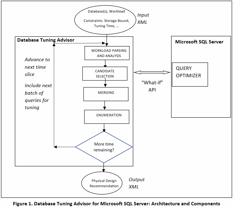
Candidate Selection (Section 4): This step is performed on one query at a time. The goal of candidate selection is to identify a good set of configurations for the query. The physical design structures in those configurations become the input to the Merging step as well as the Enumeration step.
Merging (Section 5). Candidate selection is designed to select indexes and materialized views that are optimal for the query. However, when provided with a storage bound (or limit on the number of indexes etc.), it is possible that we end up with sub-optimal recommendation for the input workload. Merging considers the space of indexes and materialized views that although are not optimal for any individual query, are useful for multiple queries, and therefore may be optimal for the workload. The output of Merging is a new set of candidate indexes and materialized views which are input to Enumeration.
Enumeration (Section 6). Enumeration does a search over all physical design structures identified by Candidate Selection and Merging, and outputs a configuration with low aggregate optimizer estimated cost for the workload that also honors all constraints described in Section [1] (e.g. the storage bound).
Scope of this article
What is covered: The algorithm overview describe above can be viewed as the “outer loop” of tuning, that is general for all physical design recommendations produced by DTA. In the rest of this article however, we will focus primarily on DTA’s algorithms for B+Tree Indexes (Clustered and Non-clustered) as well as Materialized Views. We describe each of the key modules: Workload Parsing and Analysis, Candidate Selection, Merging and Enumeration. Finally, in Section 7 we describe how the anytime property of the algorithm is realized.
What is not covered: For simplicity of exposition, we omit the following topics: (a) Implementation of the “What-if” API in the query optimizer, which is discussed in [2]. (b) Logic for deciding which multi-column statistics to create during tuning (see [7]). (c) Selection techniques for other physical design structures such as partitioning, filtered indexes and column-store indexes [9, 10]. (d) Details of workload parsing such as handling workload input from QueryStore [12] and plan cache, handling of cursors, queries referencing temp tables, and prepared queries.
Workload Parsing and Analysis
Parsing: In DTA, the workload can be specified in different ways: (a) A trace of queries and updates that execute against the database (e.g. using SQL Server Profiler or XEvents [15]). (b) A .sql file containing SQL statements (c) Query Store [12] (d) Plan Cache. This module analyzes each statement and extracts all relevant information from the statement required for tuning in a parsing step. This information includes tables, selection and join predicates, group by and order by columns etc. occurring in the query.
Interesting table-subsets and column-groups: Once queries are parsed, they are then mined to identify interesting table-subsets and column-groups. A table-subset (resp. column-group) is a set of tables (resp. columns) referenced in one or more queries in the workload. A column-group is restricted to be on columns from the same table. A table-subset (resp. column-group) is defined to be interesting if the total cost of all queries in which it occurs exceeds a given fraction f (a configurable parameter, with a default setting of 0.05) of the total cost of all queries in the workload. In other words, a table-subset must appear either in one or more expensive queries or must be occur in many less expensive queries to become interesting. DTA limits its tuning of indexes and materialized views to interesting table-subsets and column-groups. Materialized views are only considered on interesting table-subsets, and multi-column indexes only considered on interesting column-groups. This technique can be effective for large workloads, allowing DTA to find very good recommendations early in the tuning process. The computation of table-subsets and column-groups is done in a bottom-up manner as described in [4, 6].
Workload Compression: The goal of workload compression is to reduce the running time of DTA without compromising the quality of recommendation when the input workload is large. The algorithm is a simplified version of the techniques described in [5]. We generate a signature for each parsed statement in the workload, which is an encoding of the structure of the statement and includes the tables, predicates (without constants), group-by columns, order-by columns. For example, two queries that are different invocations of the same stored procedure or prepared statement will have identical signatures. Queries are grouped by signature. Within each group DTA randomly samples a subset of queries for tuning. The number of queries sampled is max (p, (√ ), where p is a configurable constant (default 25), and n is the number of queries in the workload. To account for the queries that are not chosen for tuning, the weight of each ignored query is added to the weight of the “nearest” query instance that is chosen for tuning -- in particular, the instance with the closest optimizer estimated cost.
Candidate Selection
DTA finds best configurations for a given query Q consisting of indexes only, followed by configurations consisting of indexes and materialized views.
Syntactically Relevant Indexes: DTA generates a set of syntactically relevant indexes for the query, i.e. those indexes that can potentially be useful for the query as described in [1]. However, there are a few modifications. First, multi-column clustered and non-clustered indexes are restricted to those defined on interesting column-groups only. Second, DTA treats columns in different clauses of the query, such as selection, join, group by and order by differently. For indexes on selection columns, DTA orders the columns by estimated selectivity of the predicate on that column. Selectivity is estimated using the histogram on that column available in SQL Server metadata catalogs. For order by columns, DTA uses the ordering specified in the query. For join predicates, DTA considers multiple indexes, one each per join column as the leading column. Finally, DTA also considers a set of covering indexes, i.e. indexes that contain all referenced columns in the query. The logic for ordering the key columns in a covering indexes is similar to the logic for non-clustered indexes described above. The columns that occur only as a projection column in the query or in scalar aggregates (e.g. SUM(X)), are added as INCLUDE columns (i.e. non-key columns) of the index.
To search for the top k configurations, DTA identifies several “seed” configurations for the query, and then invokes the Enumeration algorithm described in Section 6 on each seed configuration, passing in the syntactically relevant indexes. There are two classes of interactions considered for generation of seed configurations: indexes on join columns from two or more tables. For example, if R.A = S.B is a join predicate in the query, then indexes on R (clustered and non-clustered, including covering indexes) with R.A as the leading column and indexes on S with S.B as the leading column are considered and each such combination becomes a potential seed. A second class of interactions is for indexes on columns in selection predicates. DTA makes a single optimizer call with all non-covering non-clustered indexes on each table. The indexes chosen by the query optimizer on each table are grouped into a seed configuration.
Space of Materialized Views: For each interesting table-subset that occurs in Q, DTA considers multiple materialized view alternatives. It considers four classes: (a) Select-Project-Join (SPJ) (b) Project-Join (PJ)
- SPJG (d) PJG. These materialized views are added to a single configuration C, and the query Q is 5
optimized using the “what-if” API. The materialized views selected by the optimizer are chosen as candidates. In many cases the optimizer will prefer the SPJ or SPJG view since it is most specific to the query and is likely to be the cheapest. Hence, if either of these kinds of views are picked by the optimizer, then DTA makes an additional optimizer call by only including the more general views (i.e.) PJ and PJG classes. If the optimizer picks one of these views and the cost is within a small threshold t (default value of 5%) of the cost of the plan that uses the specific views, then DTA only chooses as candidates the more general views. This is because more general views are typically more applicable across queries in the workload.
In addition to the materialized view itself, DTA also considers a set of non-clustered indexes on each candidate materialized view. Single-column non-clustered indexes are considered on columns in the projection list of the view which occur in a selection condition. If there are tables in the query that are not part of the view, then indexes on the join columns of the query that are in the projection list of the view are also considered. This can enable plans that join the view with other tables in the query using indexes. Similarly, for SPJ and PJ view, then multi-column indexes on group-by and order-by columns in the query on projection columns in the view are considered. Any such non-clustered indexes on the candidate materialized views used by the optimizer are considered candidates.
Merging
Indexes: The details of the index merging algorithm are described in [3] (see Sections 3.3. and 3.4). The input is a set of candidate indexes S, and the output is a set of merged indexes M. For each pair of indexes in S on the same table, we consider whether that pair of indexes (I1 and I2) can be merged. The merging step considers a new index I12. DTA considers only index preserving merges, i.e. the order of key columns in I12 is determined by picking the sequence of key columns of one of the two indexes (say I1) to be the leading columns of I12 and appending the sequence of key columns of the other index (I2) that are not already part of I1. The idea is that the Index Seek benefits of using at least one of the indexes are preserved, and the Index Scan benefits of using the both indexes are partially preserved (Scan benefits of both indexes may degrade since more columns than needed for the query may be scanned). DTA picks the index with higher total Index Seek benefit, i.e. the total benefit of all queries where that index is used for seeking, to contribute the leading columns in I12. Among all pairs of merged indexes, DTA greedily picks the merged index that reduces storage space the most compared to the sum of storage of its parents. It adds the merged index to M and removes the parents from S and repeats the process until no more merging is possible.
Materialized Views: The algorithm for View Merging used in DTA in described in-depth in [4] (see Section 4.3). One detail is that when two views MV1 and MV2 are merged, we need to consider non-clustered indexes on the merged view MV12. DTA preserves all non-clustered indexes on MV1 and MV2 that are still valid on MV12.
Enumeration
DTA takes an input a set of candidate indexes and materialized views C, a set of “seed” configurations S. DTA runs several greedy search algorithms, one per seed configuration. A seed configuration is designed to capture important interactions between physical design structures that might be overlooked by the greedy strategy. Seed configurations are determined during the Candidate Selection and Merging steps. Unlike the algorithm in [1], which uses seed configurations of size 2 by considering each pair of candidate indexes, DTA can consider seed configurations where the number of indexes (or physical design structures in general) can be ≥ 2. This has the dual purpose of capturing larger interactions, while also avoiding certain wasteful combinations of size
The final greedy search of DTA is done with all physical design structures considered together as described in [4]. This is important to capture interactions between indexes and materialized views. By searching over the space of candidates together, we avoid problems that arise when search is conducted separately for indexes and materialized views. For instance, an index that is chosen may no longer be used by the optimizer once a materialized view is picked.
Anytime Property
The input to DTA can sometimes be a large workload (e.g. a trace of all statements executed against the database for a week), and/or complex queries. Making “What-if” optimizer calls and creating statistics can be expensive operations. In such cases, DTA can take a significant amount of time to tune the workload. DBAs often would like to run DTA so that they complete tuning within a specified time-bound (e.g. a batch window). Furthermore, the user may want to stop the tuning after some time. Therefore, DTA’s algorithm must have the anytime property: it should ideally find a good recommendation very quickly, and progressively find better configurations if more time is provided. To address this requirement at each step during tuning, DTA must make judicious tradeoffs such as: (1) Parsing and analyzing more queries vs. tuning the parsed queries. (2) During candidate selection, continue tuning the current query vs. switch to another query. (3) It should preserve relevant state from one time slice to the next so as to minimize redundant work.
DTA achieves the anytime property using the following techniques. As noted in Section [2], DTA internally divides its work into time slices. The time allotted to each time slice is a configurable parameter. By default, DTA picks each time slice to be 15 minutes or √ (whichever is larger) where T is the total tuning time provided to DTA. In each time slice, DTA ensures that each of the major modules are provided a minimum guaranteed percentage of the time: (a) Workload Parsing and Analysis (w%) (b) Candidate selection (c%) (c) Merging and Enumeration combined (e%), with Merging never consuming more than half the time. Once again, w, c, e are configurable parameters that add up to 100%, with default values of 20, 40 and 40 respectively, which has proven effective in practice. Thus, each of DTA’s modules has built-in timers that tracks the elapsed time and has the ability to return when time runs out. If any module completes prior to its allotted time, the excess time gets distributed to the remaining steps equally.
Figure 2 shows some of the important data structures used in the DTA that are important for achieving the anytime property. The data structures are designed to be incrementally updateable and carry forward relevant state across time slices.
During the Workload Parsing and Analysis step, DTA starts consuming the workload in the order described below. If the input workload contains information about duration (i.e. execution time) of the queries, then DTA tunes queries in descending order of duration, thereby focusing on more expensive queries first. For example, duration information is available when using Microsoft SQL Server’s XEvent/Profiler tracing tools to log the workload or using the Query Store or plan cache. Otherwise, DTA uses the order of queries as specified in the input workload file. Furthermore, it focuses tuning efforts on queries in the compressed workload (as described in Section 3). This allows DTA to cover tuning of a few queries spanning many distinct query templates, before it tunes queries belong to one template exhaustively. DTA incrementally parses more queries in each time slice ensuring that it leaves sufficient time for workload compression and steps for table-subset and column-group computation. These are stored in lattice data structures to be used during candidate selection. At the end of each time slice, DTA computes a recommendation for a prefix of the workload parsed thus far.
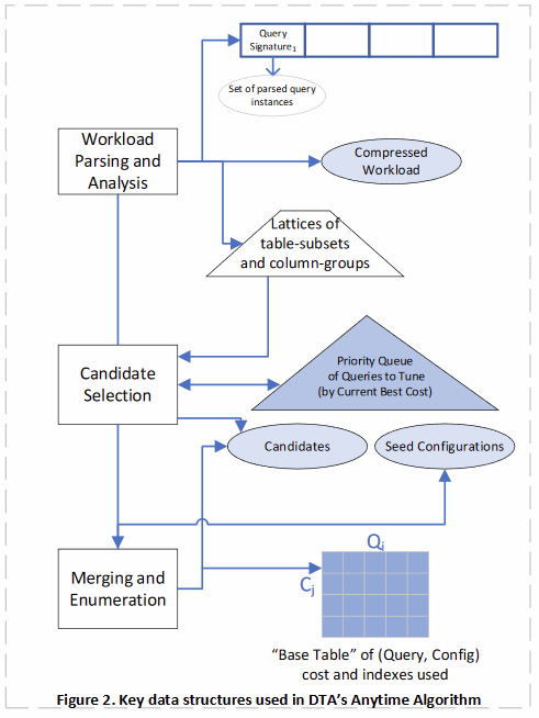
DTA maintains a priority queue of parsed and compressed queries ordered by the cost of the best configuration found for the query thus far. During candidate selection the current most expensive query Q is picked next for tuning. The table-subset with the current highest-cost that is relevant for Q is considered next and tuned for indexes and materialized views (as described in Section 4). Once the query is tuned for that table-subset, it is re-inserted into the priority queue with the cost of the best configuration found for the query thus far. The process is then repeated until time for candidate selection runs out. By using this approach, once a good set of physical design structures are found as candidates for the query, it allows tuning to switch to a different (and now more expensive) query. Once all table-subsets for a query are exhausted, the query is marked as tuned and removed from the priority queue.
DTA maintains a sparse matrix called the “Base Table” that stores the result of all “What-If” optimizer calls made thus far, and serves as a cache. A cell in this matrix contains the cost of query Qi under configuration Cj as well as all physical design structures used in the plan. Since optimizer calls can be expensive, during candidate selection, merging and enumeration, DTA consults this matrix to avoid making redundant optimizer calls. DTA operates within a limited memory budget, so if the number of cells in the matrix becomes too large, DTA gracefully spills cells to disk and brings them back in on-demand.
Before returning the final recommendation to the user DTA performs a full sweep of all queries that it parsed in the workload. For each query, it calls the query optimizer to get the plan and cost of that query for both the current configuration C and the recommended configuration Cnew. In case any physical design is not used for any of the parsed queries in the workload, it is dropped from the final recommendation. The sweep allows DTA to provide detailed reports of the impact of the recommended configuration on the workload, including estimated improvement in workload cost, index usage reports etc. To ensure that there is sufficient time for the sweep, DTA maintains an estimate of how long the sweep will take. Note that the time for the sweep increases as more queries are parsed in each time slice. At the end of a time slice, if the remaining time is less than or equal to the estimated time for the sweep, DTA stops further tuning and switches to the final sweep.
Acknowledgements
Several people have contributed deeply to the design and implementation of DTA over the years. In particular, we would like to acknowledge the contributions of: Sanjay Agrawal, Manoj Syamala, Sudipto Das and Gaoxiang Xu. We would also like to thank the SQL Server team for making the necessary changes to the database engine, developing the GUI, and developing infrastructure for automatic tuning in Azure SQL Database.
References
- Chaudhuri, S. and Narasayya, V.R., 1997, August. An efficient, cost-driven index selection tool for Microsoft SQL server. In VLDB (Vol. 97, pp. 146-155).
- Chaudhuri, S. and Narasayya, V., Microsoft Corp, 2001. What-if index analysis utility for database systems. U.S. Patent 6,223,171.
- Chaudhuri, S. and Narasayya, V., 1999, March. Index merging. In Proceedings 15th International Conference on Data Engineering (Cat. No. 99CB36337) (pp. 296-303). IEEE.
- Agrawal, S., Chaudhuri, S. and Narasayya, V.R., 2000, September. Automated selection of materialized views and indexes in SQL databases. In VLDB (Vol. 2000, pp. 496-505).
- Chaudhuri, S., Gupta, A.K. and Narasayya, V., 2002, June. Compressing sql workloads. In Proceedings of the 2002 ACM SIGMOD international conference on Management of data (pp. 488-499).
- Agrawal, S., Narasayya, V. and Yang, B., 2004, June. Integrating vertical and horizontal partitioning into automated physical database design. In Proceedings of the 2004 ACM SIGMOD international conference on Management of data (pp. 359-370).
- Agrawal, S., Chaudhuri, S., Kollar, L., Marathe, A., Narasayya, V. and Syamala, M., 2005, June. Database tuning advisor for Microsoft SQL Server 2005. In Proceedings of the 2005 ACM SIGMOD international conference on Management of data (pp. 930-932).
- Chaudhuri, S. and Narasayya, V., 2007, September. Self-tuning database systems: a decade of progress. In Proceedings of the 33rd international conference on Very large data bases (pp. 3-14).
- https://cloudblogs.microsoft.com/sqlserver/2017/01/10/announcing-columnstore-indexes-and-query-store-support-in-database-engine-tuning-advisor/
- Performance Improvements using Database Engine Tuning Advisor (DTA) recommendations. https://docs.microsoft.com/en-us/sql/relational-databases/performance/performance-improvements-using-dta-recommendations?redirectedfrom=MSDN&view=sql-server-ver15
- Dziedzic, A., Wang, J., Das, S., Ding, B., Narasayya, V.R. and Syamala, M., 2018, May. Columnstore and B+ tree-Are Hybrid Physical Designs Important?. In Proceedings of the 2018 International Conference on Management of Data (pp. 177-190).
- Monitoring Performance by using the Query Store. https://docs.microsoft.com/en-us/sql/relational-databases/performance/monitoring-performance-by-using-the-query-store?view=sql-server-ver15
- Das, S., Grbic, M., Ilic, I., Jovandic, I., Jovanovic, A., Narasayya, V.R., Radulovic, M., Stikic, M., Xu, G. and Chaudhuri, S., 2019, June. Automatically indexing millions of databases in microsoft azure sql database. In Proceedings of the 2019 International Conference on Management of Data (pp. 666-679).
- Automatic Tuning in Azure SQL Database and Azure SQL Managed Instance. https://docs.microsoft.com/en-us/azure/azure-sql/database/automatic-tuning-overview
- Extended Events (XEvents) Overview. https://docs.microsoft.com/en-us/sql/relational-databases/extended-events/extended-events?view=sql-server-ver15